Notes

Notes, Ma 191c: Pre-minimalism Linguistic Models

August 23, 2026

[lecture 2]

Transformational grammar (Chomsky, 1957).

Sentences have

  1. Deep structure (closer to semantics): represents the sentence as a tree.
  2. Surface structure (language-specific) represents the sentence as a tree after some transformations.

Example 2.8. Consider the sentence

John eats the apple.

1. Deep structure represents the sentence using a tree (imprecise, but bear with this):

S NP VP John V NP eats the apple

2. Transformational grammar equips us with a couple of pre-built transformations that we can use on this tree (passivization, question formation, negation, movement, etc.). The point of these transformations is to produce a list of related sentence-trees and say they are equivalent:

John eats the apple.
The apple was eaten by John.
Did John eat the apple?
Was the apple eaten by John?

This approach enables us to create tree families that represent the same semantic idea. The tree-representations for each of these are surface structure.

One might ask, “why did we pick John eats the apple as the deep structure tree?” We actually did not; we just made some universal assignments:

EATER=JohnEATEN THING=apple \begin{aligned} \text{EATER} &= \text{John} \\ \text{EATEN THING} &= \text{apple} \end{aligned}

and created a tree out of that; it’s just that this tree happened to look like “John eats the apple” when unrolled. The sentence tree itself is surface-level; the deep-level is this abstract assignment tree. So in general,

DeepStructuretransformsSurfaceStructure \text{DeepStructure} \xrightarrow{\text{transforms}} \text{SurfaceStructure}

There are obviously many issues with this. Here are the biggest ones in my opinion:

  1. Too many transformations.
  2. Transformation rules may not be precise.
  3. Multiple hard-coded rules.
  4. Messy when dealing with multiple languages, especially because passive transformation rules differ language-to-language.

This motivates the next idea.

Principles and parameters (Chomsky, 1981).

Two components:

  1. Principles (general grammar rules). E.g., “when building a grammar you must represent lexical word elements syntactically” (Projection Principle) or “each argument of a phrase gets one role” (θ\theta-criterion). These are true for all languages.
  2. Parameters (binary variables distinguishing different languages syntactically).

So universal principles plus language-specific parameter settings compose a specific language’s grammar. If you were to design a new language, you should note this.

Example 2.9. Let’s say “heads before complements” is a parameter. Then, for English (param=1) and Japanese (param=0) respectively, possible trees allowed by the grammar are:

VP V DP eat an apple , VP DP V ringo-o tabe

Through P&P, in an idealized world, languages are encoded as bitstrings that represent each parameter, with “general design decisions” enforced through the principles.

Example principles:

  • Structure Preservation Principle
  • Projection Principle
  • Subjacency Principle

Example parameters:

  • Head-directionality
  • Subject-side
  • Pro-drop
  • Null-subject
  • Word order (SOV, SVO, VSO, VOS, OVS, OSV)

There are a couple problems with P&P:

  1. Interdependencies between parameters. Mathematically, an aim is to figure out the “ideal set” of generators, but linguists haven’t found this yet.
  2. Changes of parameters as languages evolve (e.g., word order changes in Homeric to Classical Greek, switches from Old English to English, etc.).

Notes, Ma 191c: Mathematical Models of Generative Linguistics

August 22, 2026

[lecture 1] [lecture 2]

What is linguistics?

1. Syntax is the subset of a language’s grammar that has to do with how words legally combine into sentences. (Other subsets include morphology, which deals with how morphemes combine into words, and phonics, which deals with individual unit sounds.)

2. Language is not just a “sequence of words” because some sequences are structurally illegal. Rather, language is a “sequence of words that follows a template, paired with a hierarchy.” The hierarchy is important, as the same word-sequence with different hierarchy can constitute different sentences:

[I saw [the man with the telescope.]]
[I saw [the man][with the telescope.]]

Another example:

I shot an elephant in my pajamas.

The sentence has two possible syntactic structures.

S NP VP I V NP PP shot an elephant in my pajamas

Here, in my pajamas modifies the verb phrase: I was wearing the pajamas when I shot the elephant.

S NP VP I V NP shot NP PP an elephant in my pajamas

Here, in my pajamas modifies the noun phrase an elephant: the elephant is in my pajamas.

3. Language can be viewed as a “structure” because it is hierarchically composable. On the morpheme-level, consider:

(un-(friend)-ly))-ness

or as a tree,

N Adj -ness un- Adj N -ly friend

These trees can be further composed to give a tree structure on the whole sentence.

4. An i-language is a set of internal grammatical rules in each person’s mind. Thus, i-languages for e.g. English differ person-to-person. There is some intuitive sense of “this sentence feels right” (grammaticality) that each person has based on their specific i-language.

5. There might be some math involved in linguistics; namely, operators defined on the language-trees.

Generative linguistics: formal languages.

Formal languages describe strings of words recognizable by varying classes of automata (called Chomsky hierarchy).

Structures that give rise to formal languages:

  • Programming languages
  • Some discrete group presentations

The question: which classes of automata can recognize natural languages? A grammar is a quadruple

G=(VN,VT,P,S) \mathcal{G} = (V_N, V_T, P, S)

where

  • VNV_N and VTV_T are disjoint finite sets: non-terminal and terminal symbols, respectively.
  • SVNS \in V_N is the start symbol.
  • PP is the set of production rules, acting as a finite rewriting system on VNVTV_N \cup V_T.

The language produced by a grammar G\mathcal{G} is given by

LG={wVT:SPw} L_{\mathcal{G}} = \{w \in V_T^{\star} : S \to_P^{\star} w\}

Example 2.1. Consider grammar G=({S,A},{a,b},P,S)\mathcal{G} = (\{S, A\}, \{a, b\}, P, S) with productions:

SaAS,Sa,ASbA,ASS,AbA S \to aAS, \quad S \to a, \quad A \to SbA, \quad A \to SS, \quad A \to bA

Note that a possible word in LGL_{\mathcal{G}} is given by abaaaabaaa, since

SaASaAaabAaabSSaabSaaabaaa. S \Rightarrow aAS \Rightarrow aAa \Rightarrow abAa \Rightarrow abSSa \Rightarrow abSaa \Rightarrow abaaa.

The Chomsky hierarchy.

Type 0: unrestricted grammar, recognizable by Turing machine. Production rules are general: αβ\alpha \to \beta.

Type 1: Context-sensitive grammar, recognizable by linear bounded automaton. A context-sensitive grammar is one with

βAγβαγ,with AVN,α,β,γ(VNVT),αε \beta A \gamma \to \beta \alpha \gamma, \quad \text{with } A \in V_N, \alpha, \beta, \gamma \in (V_N \cup V_T)^{\star}, \alpha \neq \varepsilon

Note that the context is fixed and just the middle part is re-written. Type 1 is a more restricted version of Type 0.

Type 2: Context-free grammar, recognizable by nondeterministic pushdown automata. Special case of context-sensitive, with β=γ=ε\beta = \gamma = \varepsilon.

Type 3: Regular grammar, recognizable by finite state automata (e.g., NFA, DFA). More restricted version of Type 2 (we’ll see why in the next example).

Generally, we find that

Type 3Type 2Type 1Type 0 \text{Type 3} \subseteq \text{Type 2} \subseteq \text{Type 1} \subseteq \text{Type 0}

in terms of expressive power.

Example 2.2 (Context-sensitive grammar). Consider the context-sensitive grammar G=({S,B,C},{a,b,c},P,S)\mathcal{G} = (\{S, B, C\}, \{a, b, c\}, P, S), with production rules

SaSBC,SaBC,CBBC,aBab,bBbb,bCbc,cCcc \begin{aligned} S &\to aSBC, \quad S \to aBC, \quad CB \to BC, \\ aB &\to ab, \quad bB \to bb, \quad bC \to bc, \quad cC \to cc \end{aligned}

Then, we find possible strings are

  • SaBCabCabcS \Rightarrow aBC \Rightarrow abC \Rightarrow abc
  • SaSBCaaBCBCaabCBCaabBCCaabbCCaabbcCaabbccS \Rightarrow aSBC \Rightarrow aaBCBC \Rightarrow aabCBC \Rightarrow aabBCC \Rightarrow aabbCC \Rightarrow aabbcC \Rightarrow aabbcc

and in general,

LG={anbncn:n1} L_{\mathcal{G}} = \{a^n b^n c^n : n \geq 1\}

Example 2.3 (Context-free grammar). Take the context-free grammar G=({S},{0,1},P,S)\mathcal{G} = (\{S\}, \{0, 1\}, P, S) where the production rules are given by

S0S1,S01 S \to 0S1, \quad S \to 01

Then, we find possible strings are

  • 0101
  • 00110011
  • 000111000111
  • \ldots

and in general,

LG={0n1n:n1} L_{\mathcal{G}} = \{0^n 1^n : n \geq 1\}

We know this LGL_{\mathcal{G}} is not regular, because finite automata have fixed memory; remembering nn requires storing a variable.

Example 2.4 (Regular grammars). Consider G=({S,A},{0,1},P,S)\mathcal{G} = (\{S, A\}, \{0, 1\}, P, S), with production rules

S0S,SA,A1A,A1 S \to 0S, \quad S \to A, \quad A \to 1A, \quad A \to 1

It is clear this is a deterministic finite automaton:

start S A 1 0 1

with AA as a terminal state. We observe that right-linear production rules yield finite automata, as the nonterminals {S,A}\{S, A\} can be viewed as states with terminals (or ε\varepsilon) as transitions. This further cements the idea that regular grammars are constrained (right-linear) context-free grammars.

How good are CFGs at representing natural language?

We show not-context-free by highlighting cross-serial dependencies in the language. [Why cross-serial dependencies yield context-free grammars?]

Some examples of context-sensitive languages:

  • Dutch.
  • Swiss-German. Some legal sentences are of the form
wanbmxcndmy w a^n b^m x c^n d^m y

for example, “Jan säit das mer (d’chind)n^n (em Hans)m^m es huus hälfed wele (laa)n^n (hafte)m^m aastriiche.”

  • LG={xxR:x{a,b}}L_{\mathcal{G}} = \{x x^R : x \in \{a, b\}^{\star}\} (where xRx^R is the reversal of xx).

However, in general, context-sensitive grammars are overkill for representing natural languages. What is the weakest grammar able to represent natural languages?

Formal languages of finitely presented groups.

Consider a situation where the grammar is a finite group, e.g., G=G=XR\mathcal{G} = G = \langle X \mid R \rangle. Then,

LG={wX^:w=1G} L_G = \{w \in \hat{X}^{\star} : w = 1_G\}

Example 2.5. Consider G=C3=aa3=1G = C_3 = \langle a \mid a^3 = 1 \rangle. Then, X^={a,a1}\hat{X} = \{a, a^{-1}\}, and

LG={an:n0mod3} L_G = \{a^n : n \equiv 0 \mod 3\}

Example 2.6. Consider G=D8=r,sr4=s2=1,srs=r1G = D_8 = \langle r, s \mid r^4 = s^2 = 1, srs = r^{-1} \rangle. Then, X^={r,r3,s}\hat{X} = \{r, r^3, s\}, and

LG={w{r,r3,s}:w=1} L_G = \{w \in \{r, r^3, s\}^{\star} : w = 1\}

What kind of formal languages can be represented by such finite groups? Algebraic properties of GG correspond to the properties of LGL_G. Note that:

  1. LGL_G is regular iff GG is finite.
  2. LGL_G is context-free iff GG has a free subgroup of finite index.

Example 2.7. Take the infinite group G=SL2(Z)=S,TS4=I,S2=(ST)3G = SL_2(\mathbb{Z}) = \langle S, T \mid S^4 = I, S^2 = (ST)^3 \rangle, where

S=(0110),T=(1101) S = \begin{pmatrix} 0 & -1 \\ 1 & 0 \end{pmatrix}, \quad T = \begin{pmatrix} 1 & 1 \\ 0 & 1 \end{pmatrix}

We know LGL_G is not regular since GG is not finite. Consider

A=(1021),B=(1201) A = \begin{pmatrix} 1 & 0 \\ 2 & 1 \end{pmatrix}, \quad B = \begin{pmatrix} 1 & 2 \\ 0 & 1 \end{pmatrix}

Since no combination of A,BA, B equals II, it follows that F2=A,BF_2 = \langle A, B \rangle is a free group; since detA=detB=1\det A = \det B = 1, F2GF_2 \leq G.

Next, we define Γ(2)\Gamma(2) as the set of matrices congruent to I2mod2I_2 \mod 2. Since

(1021)(1001)mod2,(1201)(1001)mod2 \begin{pmatrix} 1 & 0 \\ 2 & 1 \end{pmatrix} \equiv \begin{pmatrix} 1 & 0 \\ 0 & 1 \end{pmatrix} \mod 2, \quad \begin{pmatrix} 1 & 2 \\ 0 & 1 \end{pmatrix} \equiv \begin{pmatrix} 1 & 0 \\ 0 & 1 \end{pmatrix} \mod 2

it follows that A,BΓ(2)A, B \in \Gamma(2).

We define π:SL2(Z)SL2(F2)\pi : SL_2(\mathbb{Z}) \to SL_2(\mathbb{F}_2), with kerπ=Γ(2)\ker \pi = \Gamma(2). By the First Isomorphism Theorem,

SL2(Z)/Γ(2)SL2(F2) SL_2(\mathbb{Z})/\Gamma(2) \cong SL_2(\mathbb{F}_2)

so [SL2(Z):Γ(2)]=SL2(F2)=6[SL_2(\mathbb{Z}) : \Gamma(2)] = |SL_2(\mathbb{F}_2)| = 6. Similarly, since Γ(2)=F2IF2\Gamma(2) = F_2 \sqcup -IF_2, [Γ(2):F2]=2[\Gamma(2) : F_2] = 2, and [SL2(Z):F2]=[SL2(Z):Γ(2)][Γ(2):F2]=(6)(2)=12[SL_2(\mathbb{Z}) : F_2] = [SL_2(\mathbb{Z}) : \Gamma(2)][\Gamma(2) : F_2] = (6)(2) = 12. Since GG has a free subgroup HH of finite index, LGL_G is context-free.

This section just shows that there is a nice tie between groups and languages. It doesn’t mean we have to use them over production rules.

Boundaries of Babel problem.

How do we formally characterize the space of natural languages? It is between context-sensitive and context-free. What is the geometry of this space? (Geometry basically means we represent each language as a point, with dimensions such as “head size.”)

We want a formal model to describe natural languages. Formal languages are no longer viewed a good way to model generative syntax.

  • They focus on strings rather than structures. Remember that the same string can have different meanings based on the hierarchy. Only focusing on the strings means that the hierarchy information is not generated.
  • The production rules get too complicated.
  • There are too many languages in the context-sensitive class that are not natural languages.
Stage 1: string problem
CFGs are too weak for some natural-language dependencies

need mildly context-sensitive power
Stage 2: structure problem
Knowing which strings are legal isn't enough

need a theory that actually generates syntactic structures

So, context-sensitive grammar is more powerful about strings, not automatically better about trees.

Notes on Graph Pebbling (continued)

July 16, 2026

tt-reachability, tt-pebbling number.

Let GG be a connected graph, and rV(G)r \in V(G) be the root with CC as a pebble configuration. A vertex rr is tt-reachable under CC if there is a sequence of ordinary pebbling moves after which C(r)tC(r) \geq t. Equivalently, CC is tt-fold rr-solvable. (Notice that 1-reachable is simply rr-solvable.)

Example 2.1. Consider G=P3G = P_3, with root r=v2r = v_2 and all pebbles starting at v0v_0. We recall that moving 1 pebble from v0v_0 to v2v_2 requires 4 initial pebbles. To end with C(v2)=2C(v_2) = 2, we follow the path:

(8,0,0)(0,4,0)(0,0,2) (8, 0, 0) \mapsto (0, 4, 0) \mapsto (0, 0, 2)

Generally, we conjecture that from a single pile vv at distance dd from the root, moving tt pebbles to the root requires C(v)(t)(2n)C(v) \geq (t)(2^n).

Notice that (n+1)(n+1)-reachability implies nn-reachability.

Definition 2.1. We define πt(G)\pi_t(G) as the smallest integer kk such that every configuration of kk pebbles is tt-fold rr-solvable for all rV(G)r \in V(G). Note that π1(G)=π(G)\pi_1(G) = \pi(G).

Example 2.2 (Trivial P2P_2 example). We compute π2(P2)\pi_2(P_2). Clearly, π2(P2)>2\pi_2(P_2) > 2 (consider C=(1,1)C = (1, 1)). Fix r=v1r = v_1; then, (3,0)(3, 0) is not 2-fold rr-solvable, so π2(P2)>3\pi_2(P_2) > 3. Since (4,0),(3,1),(,2)(4, 0), (3, 1), (\ast, \geq 2) are the remaining configurations and 2-fold v2v_2-solvable, P2P_2 is 2-fold v1v_1-solvable. Reversing the direction generalizes to all of P2P_2. Hence, π2(P2)=4\pi_2(P_2) = 4.

Notes on Graph Pebbling

July 14, 2026

Ordinary graph pebbling.

Graph pebbling (now a famous mathematical game) was originally introduced to solve the Erdős–Lemke conjecture: given an integer sequence a1,a2,,ana_1, a_2, \ldots, a_n, there exists a subsequence whose sum is divisible by nn, provided

i=1ngcd(ai,n)n \sum_{i=1}^{n} \gcd(a_i, n) \geq n

Now, let G=(V,E)G = (V, E) be a connected graph.

Definition 1.1 (Configuration). A configuration is an assignment C:VZ0C : V \to \mathbb{Z}_{\geq 0}, where C(v)C(v) is the number of pebbles placed at vertex vv.

Definition 1.2 (Pebbling move). A pebbling move from vertex uu to an (adjacent) vertex vv does two things:

  1. C(u)C(u)2C(u) \mapsto C(u) - 2
  2. C(v)C(v)+1C(v) \mapsto C(v) + 1

Thus, moving a pebble across an edge has a cost; the total pebbles in GG are decreased by 1.

Example 1.1. Consider the path graph P3P_3:

v0 v1 v2

Suppose all pebbles are at v0v_0. To place 1 pebble at v1v_1, we need at least 2 pebbles in v0v_0. To place 1 pebble at v2v_2, we need at least 2 pebbles in v1v_1, and therefore 4 pebbles in v0v_0.

Example 1.2. Consider P4P_4. Defining “arrival” at vertex vv as having 1 pebble in vv, we find:

Vertex Pebbles needed to guarantee arrival
v0v_0 1
v1v_1 2
v2v_2 4
v3v_3 8

It seems 2k2^k pebbles are needed to reach vkv_k (if all pebbles start at v0v_0) for a path graph Pk+1P_{k+1}.

Example 1.3 (Reachability depends on the configuration). Consider P3P_3, with C(v0)=3,C(v1)=0,C(v2)=0C(v_0) = 3, C(v_1) = 0, C(v_2) = 0. v2v_2 is not reachable; (C(v0),C(v1),C(v2))=(3,0,0)(1,1,0)(C(v_0), C(v_1), C(v_2)) = (3, 0, 0) \mapsto (1, 1, 0) which is a terminal state.

However, v2v_2 is reachable under (2,1,0)(0,2,0)(0,0,1)(2, 1, 0) \mapsto (0, 2, 0) \mapsto (0, 0, 1). Both configurations have 3 total pebbles. This emphasizes that reachability depends not only on total pebbles in GG, but the specific configuration.

Definition 1.3 (rr-solvable). Choose a target vertex rr, called the root. A configuration CC is rr-solvable when a sequence of pebbling moves puts at least 1 pebble in vertex rr. E.g., in the previous example, the first configuration was not v2v_2-solvable but it was v1v_1-solvable. Thus solvability depends on the configuration and the chosen root.

Definition 1.4 (Pebbling number). The pebbling number π(G)\pi(G) is the smallest integer kk such that every configuration of kk pebbles CkC_k is rr-solvable for all rV(G)r \in V(G).

Note that to prove π(G)k\pi(G) \leq k, we must prove that every CkC_k is rr-solvable rV(G)\forall r \in V(G), whereas to prove π(G)>k\pi(G) > k, we must show there exists a configuration CkC_k that is not rr-solvable for some rV(G)r \in V(G).

Example 1.4 (Computing π(P3)\pi(P_3)). In this example, we explicitly compute π(P3)\pi(P_3).

Proof. We can immediately establish a lower bound from the previous example; since there exists C3=(3,0,0)C_3 = (3, 0, 0) that is not v2v_2-solvable, π(P3)>3\pi(P_3) > 3.

Because C4=(4,0,0)C_4 = (4, 0, 0) can reach v2v_2 (the furthest vertex), it is a reasonable conjecture that π(P3)=4\pi(P_3) = 4. However, we must confirm that every 4-pebble configuration can reach every root. Starting with r=v2r = v_2: we know the (,,1),(,2,),(4,0,0)(\ast, \ast, \geq 1), (\ast, \geq 2, \ast), (4, 0, 0) configurations are v2v_2-solvable. This leaves (3,1,0)(3, 1, 0), which is solvable through the sequence (3,1,0)(1,2,0)(1,0,1)(3, 1, 0) \mapsto (1, 2, 0) \mapsto (1, 0, 1). Hence, P3P_3 is v2v_2-solvable. (The same logic applies for v0v_0, which can be viewed as an endpoint by reversing P3P_3.)

Finally, we must check if P3P_3 is v1v_1-solvable. Immediately, we know that (2,,),(,,2),(,1,)(\geq 2, \ast, \ast), (\ast, \ast, \geq 2), (\ast, \geq 1, \ast) are v1v_1-solvable. These cover all possible cases; thus, P3P_3 is v1v_1-solvable.

Hence, π(P3)=4\pi(P_3) = 4. \square

Relativity (Escher)

June 18, 2026

Aim: Design a perspective-based game where:

  1. The player initially doesn’t know the rules and must figure them out.
  2. If the player knows the rules, the game is trivial.
  3. Level nn introduces a counterexample to what the player thinks the goal is.

The game is perspective-based because it is possible for the player to possess a sub-par world model (perspective) (i.e., one that only perfectly holds from Level 1 to ii) and still beat the game. World models are built in varying abstraction hierarchies, as shown in [1]:
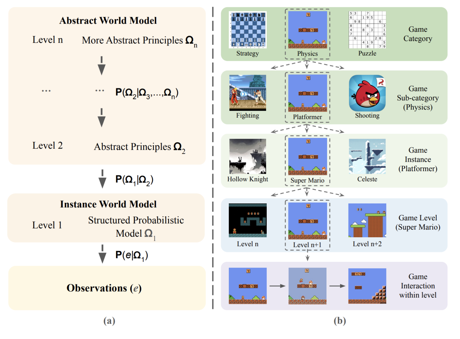
Two-panel diagram: (a) an abstraction hierarchy of world models, from observations at Level 1 up through a structured probabilistic instance model to increasingly abstract principles at Level n; (b) a parallel game hierarchy, from broad game category down through sub-category, instance, and level to interactions within a level.

This is analogous to Relativity (e.g., the staircase in one orientation is a roof in another).
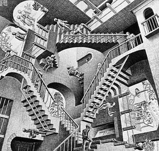
M. C. Escher, Relativity (1953) — a lithograph of staircases and figures oriented to three different gravitational directions.
Relativity, Escher [2]

https://arxiv.org/pdf/2507.12821

Loose thoughts: if a platformer, the game map might be similar to Relativity. What seems like a block in 2D could be a door in 3D; progressing across levels in 2D in a scrolling platformer is in reality walking through doors in a 3D choose your own adventure; the 3D choose your own adventure could have interesting topologies, like a Mobius strip taking you back to the start, but with different mechanics only visible in 3D (so if the player still has a 2D world model, they have to build a fake mod 2 rule that doesn't capture the real universe's mechanics).

Fugue: The orphans' crossroads (Bach, "Little" Fugue in G minor, 0:00-0:55)

June 17, 2026

An abandoned road,
Silent,
Besides the quiet footsteps,
Of two war orphans,
Walking towards each other.

A frail young boy,
Starved,
Ribcage poking through aged skin.
Bright crimson hair,
Beautiful,
Yet matted,
By the cold wind,
And lack of shelter.

An old man,
Long white beard,
And bald head,
Who only knew pain:
At age seven,
Mother's throat slit,
In the living room,
...Father, gutted,
Doused in gasoline,
And ignited,
By enemy troops.


The old man,
Glancing at a fellow war orphan,
Eyes him,
Smells him,
Ignores him,
And trods along the path to his village,
As countless others had done to him before.
"Learn pain," he yells silently,
"And feel what I feel.
Orphan...so? You're still a boy.
Whereas I had to endure that,
For my entire life."


The old man,
Pitying a fellow war orphan,
Clothes him,
Bathes him,
Feeds him,
And reads him stories,
As he warms in the campfire.
But what started as pity,
Grows into habit,
And soon,
Years pass,
Their bond morphing,
From stranger and stranger,
To father and son.

But alas,
The old man,
Had unfinished war duties,
To fulfill,

Without the boy.

So as Father,
Attempts to make,
His way home,
The boy grabs,
An origami rose,
From his bag,
Looks up,
With innocent eyes,
Teary,
Presenting his father with a gift.

So as Father,
Attempts to make,
His way home,
The boy grabs,
A dark steel rod,
And,
Once-again betrayed,
Pierces the old man's chest from behind,
Kicking him into the lake.


And,
After fifty long years,
The old man,
Pushing one more away,
Remains empty,
Devoid of a human heart.


And,
After fifty long years,
The old man feels content,
For he finally has,
A single soul,
To call his own.


And,
After fifty long years,
The frog,
At the bottom of the well,
Drifts off,
Into the great ocean.

GPU-Accelerated Simulated Annealing for VLSI Macro Placement

June 17, 2026

Given a rectangular chip die, a set of rectangular macros, fixed pins, and a hypergraph netlist, the program searches for a legal macro placement that minimizes estimated wirelength and overlap, with the heavy cost evaluation on the GPU.

Background. Macro placement is an important problem in chip physical design. In modern chips, large blocks such as SRAMs, analog blocks, accelerators, and IP modules must be placed on a two-dimensional die. The placement has to satisfy geometric constraints, such as keeping macros inside the die and avoiding overlap, while also optimizing objectives such as wirelength, routing congestion, and timing.

Input: a rectangular die, a set of rectangular macros (design blocks), and a set of nets (wires) connecting those macros and fixed pins. For example:

{
  "die": {"width": 1000, "height": 1000},
  "macros": [
    {"name": "m0", "width": 100, "height": 80},
    {"name": "m1", "width": 120, "height": 90}
  ],
  "pins": [
    {"name": "p0", "x": 0, "y": 500}
  ],
  "nets": [
    ["m0", "m1", "p0"]
  ]
}

The goal is to assign each macro an (x,y)(x, y) location such that the macros do not overlap and the estimated interconnect cost is low. This is well-suited for CUDA because many parts of the placement objective are parallelizable. For example, the half-perimeter wirelength of each net can be computed independently. Also, many simulated annealing chains can be run independently in parallel, allowing the GPU to explore many possible placements at once.

The program first generates an initial random placement. The CPU baseline improves the placement using simulated annealing. Then the CUDA implementation runs many annealing chains in parallel and returns the best placement found.

Computation. Each placement consists of coordinates for NN macros P={(xi,yi)}i=1NP = \{(x_i, y_i)\}_{i=1}^{N} where macro ii has width wiw_i and height hih_i. The cost function combines wirelength, overlap, and boundary penalties:

C(P)=αHPWL(P)+βOverlapPenalty(P)+γBoundaryPenalty(P) C(P) = \alpha \cdot \operatorname{HPWL}(P) + \beta \cdot \operatorname{OverlapPenalty}(P) + \gamma \cdot \operatorname{BoundaryPenalty}(P)

The half-perimeter wirelength of a net nn is:

HPWL(n)=(maxpnxpminpnxp)+(maxpnypminpnyp) \operatorname{HPWL}(n) = \left(\max_{p \in n} x_p - \min_{p \in n} x_p\right) + \left(\max_{p \in n} y_p - \min_{p \in n} y_p\right)

The total wirelength is HPWL(P)=nNHPWL(n)\operatorname{HPWL}(P) = \sum_{n \in \mathcal{N}} \operatorname{HPWL}(n) where N\mathcal{N} is the set of nets.

The overlap penalty between two macros ii and jj can be computed using their rectangle intersection area. If macro ii occupies [xi,xi+wi]×[yi,yi+hi][x_i, x_i + w_i] \times [y_i, y_i + h_i] and macro jj occupies [xj,xj+wj]×[yj,yj+hj][x_j, x_j + w_j] \times [y_j, y_j + h_j], then their overlap area is:

max ⁣(0,min(xi+wi,xj+wj)max(xi,xj))max ⁣(0,min(yi+hi,yj+hj)max(yi,yj)) \max\!\left(0, \min(x_i + w_i,\, x_j + w_j) - \max(x_i, x_j)\right) \cdot \max\!\left(0, \min(y_i + h_i,\, y_j + h_j) - \max(y_i, y_j)\right)

The total overlap penalty is:

OverlapPenalty(P)=i<joverlap(i,j) \operatorname{OverlapPenalty}(P) = \sum_{i < j} \operatorname{overlap}(i, j)

The simulated annealing algorithm proposes random moves such as moving one macro to a new location or swapping two macros. If the new placement has cost difference ΔC=C(Pnew)C(Pold)\Delta C = C(P_{\text{new}}) - C(P_{\text{old}}), then the move is accepted with probability p=min ⁣(1,eΔC/T)p = \min\!\left(1, e^{-\Delta C / T}\right) where TT is the current temperature.

The CPU version runs a single simulated annealing chain. The CUDA version runs many independent chains in parallel, each starting from a different random initial placement. At the end, the program chooses the best placement among all chains.

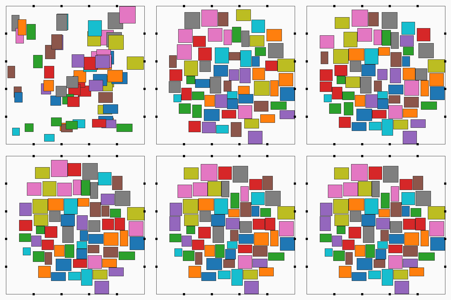
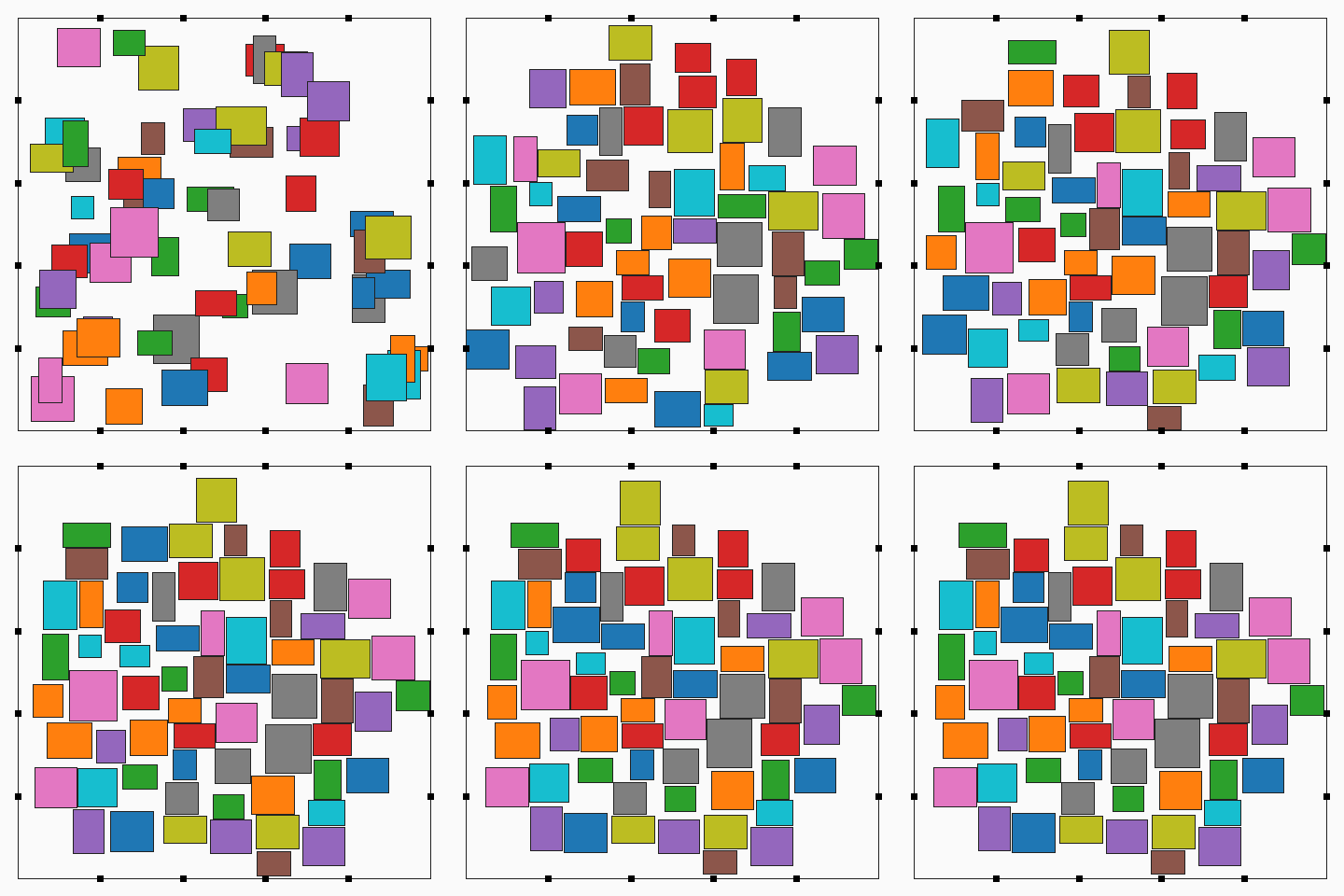
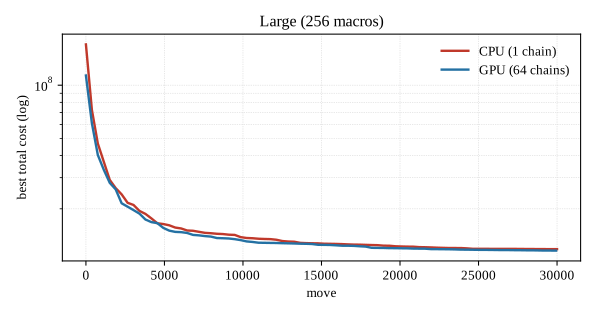
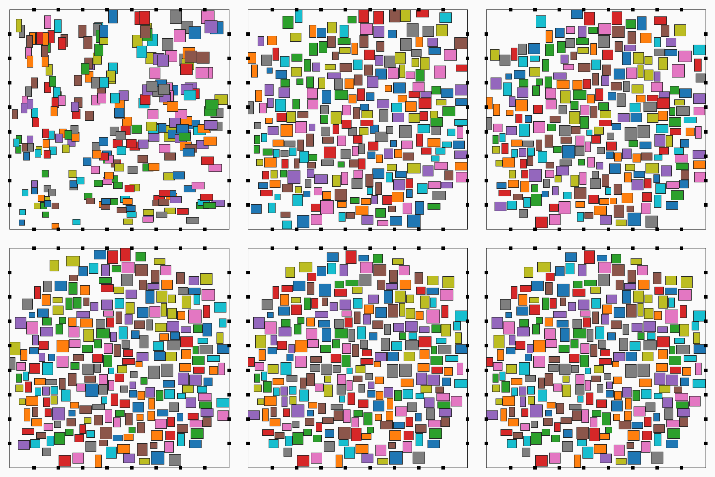
Results. Each synthetic benchmark below uses the same SA schedule (TT from 100100 to 0.0010.001, cooling 0.9950.995, 30,00030{,}000 moves, seed 4242) and the same random initial placement per size. The CPU baseline runs a single annealing chain; the GPU implementation runs 6464 independent chains and keeps the best.

Benchmark Macros Nets Die CPU total GPU total CPU time GPU time Speedup
Small 8 20 1000×1000 15,145 15,086 124 ms 510 ms 0.24×
Medium 64 200 4000×4000 796,481 755,343 3,474 ms 1,241 ms 2.80×
Large 256 1000 10000×10000 11,826,771 11,603,684 44,758 ms 12,761 ms 3.51×

The GPU pays off once the problem is large enough to amortize kernel-launch and transfer overhead: it is ~2.8× faster at medium and ~3.5× faster at large, while also reaching a slightly lower final cost (more chains explore more of the space). On the tiny 8-macro problem the GPU is slower than the CPU (0.24×) — there isn’t enough work to hide the overhead.

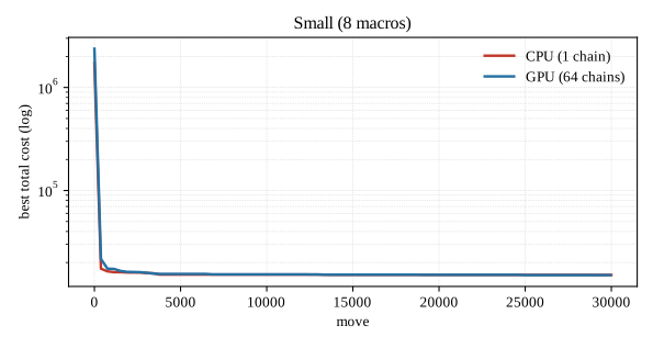
Small benchmark. 8 macros, 20 nets, 1000×1000 die. Both solvers cut the cost ~99% with zero overlap and zero boundary violation.

Metric CPU GPU
Total cost 15,144.77 15,085.94
HPWL 15,144.77 15,085.94
Overlap 0.00 0.00
Boundary 0.00 0.00
Improvement 99.12% 99.13%
Runtime 124.2 ms 510.1 ms
Convergence: CPU vs GPU, small benchmark
Best total cost vs. move (log scale).
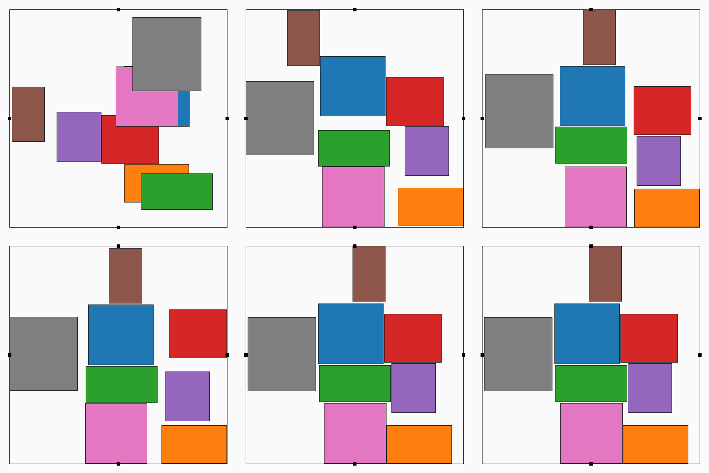
CPU convergence, small benchmark
CPU (1 chain)
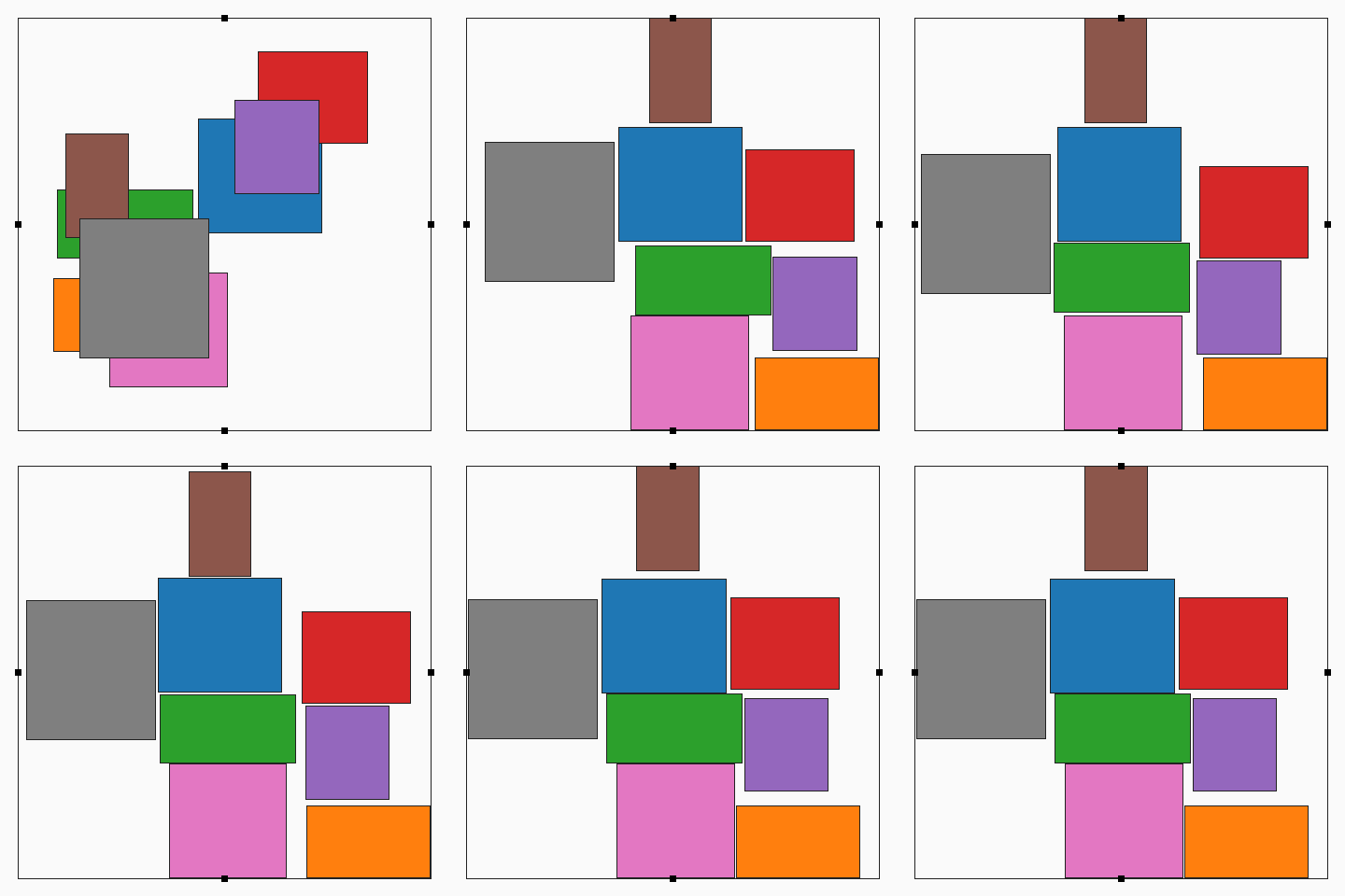
GPU convergence, small benchmark
GPU (64 chains)

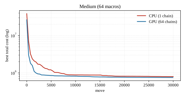
Medium benchmark. 64 macros, 200 nets, 4000×4000 die.

Metric CPU GPU
Total cost 796,480.57 755,342.94
HPWL 796,310.11 755,104.69
Overlap 17.05 23.82
Boundary 0.00 0.00
Improvement 97.93% 98.04%
Runtime 3,474.2 ms 1,240.8 ms
Convergence: CPU vs GPU, medium benchmark
Best total cost vs. move (log scale).
CPU convergence, medium benchmark
CPU (1 chain)
GPU convergence, medium benchmark
GPU (64 chains)

Large benchmark. 256 macros, 1000 nets, 10000×10000 die.

Metric CPU GPU
Total cost 11,826,770.79 11,603,684.00
HPWL 11,814,036.77 11,597,189.00
Overlap 1,056.78 448.23
Boundary 21.66 20.13
Improvement 93.05% 93.18%
Runtime 44,757.9 ms 12,761.3 ms
Convergence: CPU vs GPU, large benchmark
Best total cost vs. move (log scale).
CPU convergence, large benchmark
CPU (1 chain)
GPU convergence, large benchmark
GPU (64 chains)

At medium and large sizes a small residual overlap remains (the penalty keeps it tiny but nonzero); the 8-macro case converges to exactly zero overlap.

Euthyphro, Plato

June 16, 2026

[book]

[1] Socrates outlines a problem with a god-given absolute piety within a polytheistic religion: are pious things pious because the gods love them, or do the gods love them because they are inherently pious?

  • The main framework for the former is divine command theory. Risk: morality becomes arbitrary.
  • Frameworks for the latter: moral realism, rationalist ethics, etc. Risk: morality is defined outside of god(s).

[2] Euthyphro’s claims are that 1) Zeus would prosecute his own father for manslaughter, 2) he is the only man who knows what the gods would do (perfect religious knowledge), and 3) Man should aspire to do what God would.

  • Socrates’ initial critique against 1) is a pushback on prosecuting one’s family. To this, Euthyphro cites Zeus, who put his father Kronos in bonds for “unjustly swallowing his sons,” and Kronos, who castrated his father Ouranos.
  • Socrates finds trouble with 3) as it requires a definition of piety and an agreement on all gods’ actions. See [3].

[3] The present situation is generalized into a debate on piety, which Socrates opens by asking for a simple definition.

  • Euthyphro’s initial definition: piety is prosecuting the wrongdoer. Socrates easily refutes this as an example of piety rather than a definition.
  • Euthyphro’s revised general definition: what is loved by the gods is pious, and what is not loved by the gods is impious (loved by the gods iff. pious).
  • Socrates points out the problem of disagreement on piety within a polytheistic framework, to which Euthyphro claims (see [1]) that on his current matter, the gods reach agreement. This implicitly re-defines piety to “what is loved by ALL gods is pious”, and impiety to “what is hated by ALL gods is impious.”
    • This breaks the biconditional: now, something can be pious without being loved by all the gods (since it no longer falls under the definition of impiety). Similarly, something can be impious without being hated by all the gods.
    • This changes Euthyphro’s “definition” of piety to an example of it (“what is loved by ALL gods” is an example of many things which are pious).
  • Socrates asks, “is the pious loved by the gods because it is pious, or is it pious because it is loved by the gods?”
    • (Biconditional can hold; good movie iff. is loved by all critics. However, is it a good movie because it is loved by all critics, or is it loved by all critics because it is a good movie? The latter is more plausible; there exists a deeper reason humans find a movie “good,” and all critics have captured it.)
    • Socrates takes a similar stance: the pious is loved by the gods because it is pious.
  • Euthyphro revises piety again: “the part of justice concerned with attending to the gods.”
    • This definition seems to be something loved by all the gods, so it is valid.
    • Socrates refutes: “what can humans give gods that they don’t already have or can get?”
    • (I disagree with Euthyphro’s slavery analogy; because humans are finite, the master puts the slave to work on tasks he does not have time or will for. This does not seem to be the form of “attending” gods would like from humans. Rather, the only thing gods cannot do (self-imposedly) is violate human free will; hence, they require attending in human belief, e.g., prayer, sacrifices, etc.)
      • Still, if piety is sacrifice/prayer that pleases the gods, then Euthyphro has circled back to “pious is what is loved by the gods.”

The meaning of life

June 4, 2026

I had to think about this question a lot when:

  1. Moving to California and forfeiting college enrollment.
  2. Living alone in Sonoma County, working to prove to parents, friends, VCs, and myself that I was exceptional.
  3. Working 16 hour days in Arcadia, ending up in the hospital (treating the people around me poorly; zero tolerance for distractions).
  4. Meeting my (former) love; sleepless nights working to afford an immigration lawyer so she wouldn’t have to leave the US.
  5. Contemplating various ethical dilemmas in business.
  6. Shutting down my second startup.
  7. My friend’s death.
  8. Quitting my first and second (well-paying) jobs.
  9. Giving up my girlfriend’s hand in marriage and coming to Caltech.
  10. Watching my ex girlfriend struggle with homelessness, solitude, and suicide; failing to get the New York Police Department to track her down.
  11. My grandfather’s death.

My experiences have shaped me into (currently) a firm existentialist. I value:

  1. Knowledge and understanding. I want to understand and imagine the mathematical ideas that lie even beyond our observable universe; what can be thought of? What can’t be computed? I want to understand the recursive structure of language; the structure of music, comedy; what is moral, just (how would various philosophers have approached my gap year?); the culty-ness of startups and universities, Girard’s mimetic theory, and organized (political?) (religious?) groups.
  2. Being special.
  3. Self-improvement. After running my second business for a couple of months I began to feel unstoppable; I was solving challenge after challenge. I know that doesn’t sound unique to business…I can’t explain this properly yet; I’ll add examples when I think of them.
  4. Love. My favorite one-liner encapsulating love is ironically from Nietzsche (Beyond Good and Evil, Aphorism 153): “That which is done out of love always takes place beyond good and evil.” 'nuff said. See this.

My chat with Sam Altman

June 1, 2026

Sam Altman speaking at an event.

I used to help out at a VC/accelerator that Sam Altman put money into. My job was to read applications and determine who gets accepted (maybe funded). I saw it as paying back gratitude to something fundamental to my journey: 1) I had participated in it before, and 2) Nick and Aili helped give me a place to live when I was relatively desperate.

I met Sam Altman a couple times but I didn’t have a solid chance to chat until SF Parc (at the accelerator). We went over my life story and planned next steps. I expected him to be super anti-college; but he gave me surprising advice: go to Caltech! He mentioned some important facts that I needed to hear at the time:

  • "Don't be afraid. The regret of watching someone else live the life that could've been you outweighs the comfort of safety."
  • "Your life is yours; not your parents', investors', friends', or strangers'. Do what you want to do, not what you feel like you should be doing."
  • "Only you have enough context to understand the best decision for yourself. Be careful and don't average advice."

Places I've lived

May 30, 2026

I moved around a lot, so everywhere I lived felt temporary (including Caltech, for the first three months). Some places I’ve lived are:

  1. Ashburn (longest)
  2. Hotel Trio, Sonoma County
  3. Arcadia House, North Berkeley
  4. Dogpatch
  5. Virginia Swan Pl, Cupertino
  6. Redberry Way, San Jose
  7. 29 Cecil Ave, San Jose (first time being responsible for a home)
  8. 324 South Baywood Ave, San Jose
  9. 524 Columbus Ave, North Beach
  10. Caltech, Pasadena (2nd longest)

Each place comes with memories, and a past version of myself; the places that are burned deepest in my heart are 1, 7, 8, 3, 2 in that order.

Notes on Character Tables

May 20, 2026

Characters are constrained by group relations.

A character table is not filled with random character values such that the row and column orthogonality relations are satisfied. Rather, each row must come from an actual representation ρ:GGL(V)\rho : G \to GL(V) so the matrices ρ(g):VV\rho(g) : V \to V must still satisfy the same group relations.

This is easiest to see for a degree-1 representation ρ:GC×\rho : G \to \mathbb{C}^\times, since χV(g)=ρ(g)\chi_V(g) = \rho(g) (gG\forall g \in G). Filling in the degree-one rows in the character table is therefore the same as computing the degree-one representations for various gGg \in G.

Example 1.1 (Degree-one characters of S3S_3). Use the presentation

S3=r,sr3=s2=1, srs=r1. S_3 = \langle r, s \mid r^3 = s^2 = 1,\ srs = r^{-1} \rangle.

Let χ1\chi_1 be a degree-one character. Then,

χ1(r3)=χ1(s2)=1    ρ1(r)3=ρ1(s)2=1    χ1(r)3=χ1(s)2=1. \chi_1(r^3) = \chi_1(s^2) = 1 \implies \rho_1(r)^3 = \rho_1(s)^2 = 1 \implies \chi_1(r)^3 = \chi_1(s)^2 = 1.

Note that possible values of ρ1(r)\rho_1(r) are 1,ω,ω21, \omega, \omega^2, and possible values of ρ1(s)\rho_1(s) are ±1\pm 1. However, the ζ3\zeta_3-values for ρ1(r)\rho_1(r) do not obey srs=r1srs = r^{-1} and thus cannot be plausible assignments within a representation ρ\rho.

Then, since ρ\rho is degree-one, ρ(g)C×\rho(g) \in \mathbb{C}^\times and commutes:

χ(srs)=χ(r1)    ρ1(s)ρ1(r)ρ1(s)=ρ1(r)1    ρ1(r)2=1, \chi(srs) = \chi(r^{-1}) \implies \rho_1(s)\rho_1(r)\rho_1(s) = \rho_1(r)^{-1} \implies \rho_1(r)^2 = 1,

so ρ1(r)=ρ1(r)2=ρ1(r)3=1\rho_1(r) = \rho_1(r)^2 = \rho_1(r)^3 = 1. Similarly, ρ1(s)=±1\rho_1(s) = \pm 1. Hence, splitting across characters, we get two possible degree one character options:

χ1={r1s1χ2={r1s1 \chi_1 = \begin{cases} r \mapsto 1 \\ s \mapsto 1 \end{cases} \qquad \chi_2 = \begin{cases} r \mapsto 1 \\ s \mapsto -1 \end{cases}

so the degree-one section of S3S_3’s character table looks like this:

classesrsize132χ1111χ2111 \begin{array}{c|c|c|c} \text{class} & e & s & r \\ \text{size} & 1 & 3 & 2 \\ \hline \chi_1 & 1 & 1 & 1 \\ \chi_2 & 1 & -1 & 1 \end{array}

The takeaway: suppose someone produces a new row for χi\chi_i of the character table and χi,χj=δij\langle \chi_i, \chi_j \rangle = \delta_{ij}, passing the orthogonality checks. This doesn’t mean the χi\chi_i row is valid; rather, χi(g)\chi_i(g) must satisfy the group relations for each gGg \in G (for degree-1, since tr(g)=ρ(g)\operatorname{tr}(g) = \rho(g)).

Note that for higher degrees, tr(g)ρ(g)\operatorname{tr}(g) \neq \rho(g), so χi(g)\chi_i(g) need not follow the group relations.

How orthogonality helps complete a table.

The previous section explained where character table rows come from: traces of genuine representations satisfying the group relations.

Orthogonality enters after we have some genuine characters in hand. Its role is to compare characters and determine what irreducible pieces they contain (the character rows must be of irreducible characters χ1,χ2,,χr\chi_1, \chi_2, \ldots, \chi_r). (How does it check irreducible?)

We can compare characters in the character table through the inner product. Because characters are consistent over conjugacy classes,

χ,ψ=1GgGχ(g)ψ(g)=1GK is a conj. classKχ(gK)ψ(gK)gKK \langle \chi, \psi \rangle = \frac{1}{|G|} \sum_{g \in G} \chi(g)\overline{\psi(g)} = \frac{1}{|G|} \sum_{K \text{ is a conj. class}} |K| \chi(g_K)\overline{\psi(g_K)} \qquad g_K \in K

Example 2.1 (Why do the conjugacy class sizes appear?). Suppose G=S3G = S_3; its conjugacy classes are

{1}, {(12),(13),(23)}, {(123),(132)}. \{1\},\ \{(12), (13), (23)\},\ \{(123), (132)\}.

Then, let χ,ψ\chi, \psi be class functions. From the definition,

χ,ψ=16gGχ(g)ψ(g)=16(χ((1))ψ((1))+χ((12))ψ((12))+χ((13))ψ((13))+χ((23))ψ((23))+χ((123))ψ((123))+χ((132))ψ((132)))=16(χ((1))ψ((1))+3χ((12))ψ((12))+2χ((123))ψ((123))). \begin{aligned} \langle \chi, \psi \rangle &= \frac{1}{6} \sum_{g \in G} \chi(g)\overline{\psi(g)} \\ &= \frac{1}{6}\Big( \chi((1))\overline{\psi((1))} \\ &\qquad + \chi((12))\overline{\psi((12))} + \chi((13))\overline{\psi((13))} + \chi((23))\overline{\psi((23))} \\ &\qquad + \chi((123))\overline{\psi((123))} + \chi((132))\overline{\psi((132))} \Big) \\ &= \frac{1}{6}\Big( \chi((1))\overline{\psi((1))} + 3\chi((12))\overline{\psi((12))} + 2\chi((123))\overline{\psi((123))} \Big). \end{aligned}

which we do by picking representatives for the one-cycles, two-cycles, and three-cycles, as χ(g)ψ(g)\chi(g)\overline{\psi(g)} is constant over them. The conjugacy class sizes appear to count up the duplicates.

How does orthogonality check irreducibility?

Example 2.2. Recall that the two degree-one characters of S3S_3 are χ1=(1,1,1)\chi_1 = (1, 1, 1) and χ2=(1,1,1)\chi_2 = (1, -1, 1). If χ1,χ2\chi_1, \chi_2 are orthogonal, i.e., if the inner product χ1,χ2=0\langle \chi_1, \chi_2 \rangle = 0, then the two characters are irreducible. We check this:

χ1,χ2=16(1(1)(1)+3(1)(1)+2(1)(1))=0 \langle \chi_1, \chi_2 \rangle = \frac{1}{6}\Big( 1(1)(1) + 3(1)(-1) + 2(1)(1) \Big) = 0

We emphasize that inner product relation χi,χj=δij\langle \chi_i, \chi_j \rangle = \delta_{ij} holds for characters only, not arbitrary class functions. The practical consequence is that we must first check if χ1,χ2\chi_1, \chi_2 are characters by mapping them onto relevant representations.

What orthogonality is really saying.

For characters χ1,χ2\chi_1, \chi_2 the fact that χ1,χ1=1\langle \chi_1, \chi_1 \rangle = 1 is not merely a coincidence; this reflects that χ1\chi_1 has only one irreducible component in common with χ1\chi_1 (since χ1\chi_1 is irreducible, that component is itself). Similarly, χ1,χ2=0\langle \chi_1, \chi_2 \rangle = 0 reflects that χ1,χ2\chi_1, \chi_2 have no irreducible components in common (and are thus orthogonal).

Example 2.3. Suppose χ=2χ1+χ2\chi = 2\chi_1 + \chi_2 and ψ=χ1+3χ2\psi = \chi_1 + 3\chi_2 are both characters. Then, by linearity,

χ,ψ=2χ1+χ2,χ1+3χ2=2χ1,χ1+3χ2+χ2,χ1+3χ2=2(1χ1,χ1+3χ1,χ2)+χ2,χ1+3χ2,χ2=2(1)+6(0)+(0)+3(1)=5 \begin{aligned} \langle \chi, \psi \rangle = \langle 2\chi_1 + \chi_2, \chi_1 + 3\chi_2 \rangle &= 2\langle \chi_1, \chi_1 + 3\chi_2 \rangle + \langle \chi_2, \chi_1 + 3\chi_2 \rangle \\ &= 2(1\langle \chi_1, \chi_1 \rangle + 3\langle \chi_1, \chi_2 \rangle) + \langle \chi_2, \chi_1 \rangle + 3\langle \chi_2, \chi_2 \rangle \\ &= 2(1) + 6(0) + (0) + 3(1) \\ &= 5 \end{aligned}

Note this is a shortcut to χ,ψ=1GgGχ(g)ψ(g)\langle \chi, \psi \rangle = \frac{1}{|G|} \sum_{g \in G} \chi(g)\overline{\psi(g)} by taking advantage of χi,χj=δij\langle \chi_i, \chi_j \rangle = \delta_{ij}. Functionally, this is the dot product of each character’s multiplicity vectors.

  • χ\chi contains 2 copies of χ1\chi_1 and one copy of χ2\chi_2.
  • ψ\psi contains 1 copy of χ1\chi_1 and 3 copies of χ2\chi_2.
  • χ,ψ\langle \chi, \psi \rangle says there are (2)(1)=2(2)(1) = 2 shared χ1\chi_1 copies and (1)(3)=3(1)(3) = 3 shared χ2\chi_2 copies for a total of 2+3=52 + 3 = 5 shared irreducible character copies.

Thus, the inner product χ,ψ\langle \chi, \psi \rangle counts the number of copies of irreducibles χ1,χ2\chi_1, \chi_2 by minim_i n_i, where each mi,nim_i, n_i is a multiplicity of χ1,χ2\chi_1, \chi_2 respectively.

What a character table tells us about a representation.

A character table does more than simply list irreducible characters. Once the irreducible rows are known, it lets us decompose the character of any representation into irreducible pieces.

Suppose

χ=m1χ1+m2χ2++mrχr \chi = m_1\chi_1 + m_2\chi_2 + \cdots + m_r\chi_r

where χ1,,χr\chi_1, \ldots, \chi_r are irreducible characters and mim_i is the multiplicity of χi\chi_i. By orthogonality,

χ,χj=i=1rmiχi, χj=i=1rmiχi,χj=mjχj,χj=mj \begin{aligned} \langle \chi, \chi_j \rangle = \left\langle \sum_{i=1}^{r} m_i\chi_i,\ \chi_j \right\rangle &= \sum_{i=1}^{r} m_i \langle \chi_i, \chi_j \rangle \\ &= m_j \langle \chi_j, \chi_j \rangle \\ &= m_j \end{aligned}

so the inner product of a character χ\chi with one of its irreducible constituents χj\chi_j is its multiplicity mjm_j.

Example 3.1. Consider the irreducible characters of S3S_3:

χ1=(1,1,1)χ2=(1,1,1)χ3=(2,0,1) \begin{aligned} \chi_1 &= (1, 1, 1) \\ \chi_2 &= (1, -1, 1) \\ \chi_3 &= (2, 0, -1) \end{aligned}

and consider the degree-4 character χ=(4,0,1)\chi = (4, 0, 1). Then,

χ,χ1=16(1(4)(1)+3(0)(1)+2(1)(1))=1χ,χ2=16(1(4)(1)+3(0)(1)+2(1)(1))=1χ,χ3=16(1(4)(2)+3(0)(0)+2(1)(1))=1 \begin{aligned} \langle \chi, \chi_1 \rangle &= \frac{1}{6}\big(1(4)(1) + 3(0)(1) + 2(1)(1)\big) = 1 \\ \langle \chi, \chi_2 \rangle &= \frac{1}{6}\big(1(4)(1) + 3(0)(-1) + 2(1)(1)\big) = 1 \\ \langle \chi, \chi_3 \rangle &= \frac{1}{6}\big(1(4)(2) + 3(0)(0) + 2(1)(-1)\big) = 1 \end{aligned}

which correspond to the multiplicity mim_i of each irreducible χi\chi_i in χ\chi. Hence, χ=χ1+χ2+χ3\chi = \chi_1 + \chi_2 + \chi_3. Checking the degrees (by plugging in the identity), we find that:

χ1(1)+χ2(1)+χ3(1)=1+1+2=4=χ(1) \chi_1(1) + \chi_2(1) + \chi_3(1) = 1 + 1 + 2 = 4 = \chi(1)

which adds up.

Note then that we immediately know χ\chi is reducible because χχ1\chi \neq \chi_1 and χ,χ1=10\langle \chi, \chi_1 \rangle = 1 \neq 0.

The next proposition goes further into character irreducibility without finding invariant subspaces.

Proposition 3.1. Suppose χ:GC\chi : G \to \mathbb{C} is the character of some representation. If χ,χ=1\langle \chi, \chi \rangle = 1, then χ\chi is irreducible. If χ,χ>1\langle \chi, \chi \rangle > 1, then χ\chi is reducible.

Proof. We know χ=i=1rmiχi\chi = \sum_{i=1}^{r} m_i\chi_i. Since χi,χj=δij\langle \chi_i, \chi_j \rangle = \delta_{ij}, χ,χ=i=1rmi2\langle \chi, \chi \rangle = \sum_{i=1}^{r} m_i^2. The only way for this to equal 1 is if exactly one mi=1m_i = 1, and the remaining mj=0m_j = 0. Thus, χ=(1)χi\chi = (1)\chi_i for some 1ir1 \leq i \leq r, implying χ\chi is irreducible.

Similarly, if χ,χ>1\langle \chi, \chi \rangle > 1, either mi=1,mj>0m_i = 1, m_j > 0, or mi>1m_i > 1, so χ\chi has more than a single irreducible χi\chi_i component and is thus reducible. \square

Example 3.2 (The character of a direct sum). Suppose (V,ρV)(V, \rho_V) and (W,ρW)(W, \rho_W) are representations with characters χV\chi_V and χW\chi_W respectively. The action on the direct sum VWV \oplus W has the representation ρVW:GGL(VW)\rho_{V \oplus W} : G \to GL(V \oplus W):

ρVW(g)=(ρV(g)00ρW(g)) \rho_{V \oplus W}(g) = \begin{pmatrix} \rho_V(g) & 0 \\ 0 & \rho_W(g) \end{pmatrix}

with character χVW(g)=tr(ρVW(g))=tr(ρV(g))+tr(ρW(g))=χV(g)+χW(g)\chi_{V \oplus W}(g) = \operatorname{tr}(\rho_{V \oplus W}(g)) = \operatorname{tr}(\rho_V(g)) + \operatorname{tr}(\rho_W(g)) = \chi_V(g) + \chi_W(g).

Then, suppose VV1V2V3V \cong V_1 \oplus V_2 \oplus V_3. This implies χ=χ1+χ2+χ3\chi = \chi_1 + \chi_2 + \chi_3. Conversely, if χV=2χ1+χ2\chi_V = 2\chi_1 + \chi_2, this implies VV has decomposition VV1V1V2V \cong V_1 \oplus V_1 \oplus V_2.

Character tables of direct products.

Suppose GG and HH are finite groups. A representation of G×HG \times H can be built from a representation of GG and a representation of HH.

Consider ρ:GGL(V)\rho : G \to GL(V) and σ:HGL(W)\sigma : H \to GL(W). On the tensor product VWV \otimes W,[1] define

(ρσ)(g,h)=ρ(g)σ(h) (\rho \otimes \sigma)(g, h) = \rho(g) \otimes \sigma(h)

Aside 4.1. An element gGg \in G acts on VV, and an element hHh \in H acts on WW. An element of G×HG \times H is a pair (g,h)(g, h). We want this pair to act on a vector space with both a VV-part and a WW-part. Call this VWV \otimes W. For now, think of its vectors as vwv \otimes w for some v,wV,Wv, w \in V, W respectively. The definition of the G×HG \times H action is then (g,h)(vw)=(gv)(hw)(g, h) \cdot (v \otimes w) = (g \cdot v) \otimes (h \cdot w) (since the action must be preserved). We observe that this is shorthand for (ρσ)(g,h)(vw)=ρ(g)(v)σ(h)(w)(\rho \otimes \sigma)(g, h)(v \otimes w) = \rho(g)(v) \otimes \sigma(h)(w).

Example 4.1 (Concrete one-dimensional example). Suppose VV and WW are both one-dimensional. Assume ρ(g)v=2v\rho(g)v = 2v and σ(h)w=w\sigma(h)w = -w. Then on vwv \otimes w,

(ρσ)(g,h)(vw)=ρ(g)vσ(h)w=2vw=2(vw) \begin{aligned} (\rho \otimes \sigma)(g, h)(v \otimes w) &= \rho(g)v \otimes \sigma(h)w \\ &= 2v \otimes -w \\ &= -2(v \otimes w) \end{aligned}

Proposition 4.1. The following character relation holds: χρσ(g,h)=χρ(g)χσ(h)\chi_{\rho \otimes \sigma}(g, h) = \chi_\rho(g)\chi_\sigma(h).

Example 4.2. The trace of a tensor product of matrices is the product of their traces,[2] so reasonably,

χρσ(g,h)=tr((ρσ)(g,h))=tr(ρ(g))tr(σ(h))=χρ(g)χσ(h) \begin{aligned} \chi_{\rho \otimes \sigma}(g, h) &= \operatorname{tr}((\rho \otimes \sigma)(g, h)) \\ &= \operatorname{tr}(\rho(g))\operatorname{tr}(\sigma(h)) \\ &= \chi_\rho(g)\chi_\sigma(h) \end{aligned}

Example 4.3 (C2×C2C_2 \times C_2). Let C2=ss2=1C_2 = \langle s \mid s^2 = 1 \rangle, with irreducible characters χ1=(1,1)\chi_1 = (1, 1) and χ2=(1,1)\chi_2 = (1, -1).

Now, consider C2×C2={(1,1),(s,1),(1,s),(s,s)}C_2 \times C_2 = \{(1,1), (s,1), (1,s), (s,s)\}. To build a character of C2×C2C_2 \times C_2, we choose an irreducible character from the first C2C_2 copy and second from the second C2C_2 copy. Then, there are four possible irreducible characters: χ1χ1,χ1χ2,χ2χ1,χ2χ2\chi_1 \otimes \chi_1, \chi_1 \otimes \chi_2, \chi_2 \otimes \chi_1, \chi_2 \otimes \chi_2. We find

(χ1χ1)(g1,g2)=χ1(g1)χ1(g2)(χ1χ2)(g1,g2)=χ1(g1)χ2(g2)(χ2χ1)(g1,g2)=χ2(g1)χ1(g2)(χ2χ2)(g1,g2)=χ2(g1)χ2(g2) \begin{aligned} (\chi_1 \otimes \chi_1)(g_1, g_2) &= \chi_1(g_1)\chi_1(g_2) \\ (\chi_1 \otimes \chi_2)(g_1, g_2) &= \chi_1(g_1)\chi_2(g_2) \\ (\chi_2 \otimes \chi_1)(g_1, g_2) &= \chi_2(g_1)\chi_1(g_2) \\ (\chi_2 \otimes \chi_2)(g_1, g_2) &= \chi_2(g_1)\chi_2(g_2) \end{aligned}

and filling out the character table,

class(1,1)(1,s)(s,1)(s,s)size1111χ1χ1(1)(1)=1(1)(1)=1(1)(1)=1(1)(1)=1χ1χ2(1)(1)=1(1)(1)=1(1)(1)=1(1)(1)=1χ2χ1(1)(1)=1(1)(1)=1(1)(1)=1(1)(1)=1χ2χ2(1)(1)=1(1)(1)=1(1)(1)=1(1)(1)=1 \begin{array}{c|c|c|c|c} \text{class} & (1,1) & (1,s) & (s,1) & (s,s) \\ \text{size} & 1 & 1 & 1 & 1 \\ \hline \chi_1 \otimes \chi_1 & (1)(1) = 1 & (1)(1) = 1 & (1)(1) = 1 & (1)(1) = 1 \\ \chi_1 \otimes \chi_2 & (1)(1) = 1 & (1)(-1) = -1 & (1)(1) = 1 & (1)(-1) = -1 \\ \chi_2 \otimes \chi_1 & (1)(1) = 1 & (1)(1) = 1 & (-1)(1) = -1 & (-1)(1) = -1 \\ \chi_2 \otimes \chi_2 & (1)(1) = 1 & (1)(-1) = -1 & (-1)(1) = -1 & (-1)(-1) = 1 \end{array}

Example 4.4 (S3×S3S_3 \times S_3). As another example, we consider S3×S3S_3 \times S_3. Taking the irreducible characters from S3S_3, we find:

χ1(g)=1χ2(g)=sgn(g)χ3(g)=(2,0,1) \begin{aligned} \chi_1(g) &= 1 \\ \chi_2(g) &= \operatorname{sgn}(g) \\ \chi_3(g) &= (2, 0, -1) \end{aligned}

We partially complete the S3×S3S_3 \times S_3 character table.

classes(1,1)(1,2)(1,3)(2,1)(2,2)(2,3)(3,1)(3,2)(3,3)size132396264χ1χ1111111111χ1χ2(1)(1)(1)(1)(1)(1)(1)(1)(1)(1)(1)(1)(1)(1)(1)(1)(1)(1)χ1χ3χ2χ1χ2χ2χ2χ3χ3χ1χ3χ2χ3χ3 \begin{array}{c|c|c|c|c|c|c|c|c|c} \text{classes} & (1,1) & (1,2) & (1,3) & (2,1) & (2,2) & (2,3) & (3,1) & (3,2) & (3,3) \\ \text{size} & 1 & 3 & 2 & 3 & 9 & 6 & 2 & 6 & 4 \\ \hline \chi_1 \otimes \chi_1 & 1 & 1 & 1 & 1 & 1 & 1 & 1 & 1 & 1 \\ \chi_1 \otimes \chi_2 & (1)(1) & (1)(-1) & (1)(1) & (1)(1) & (1)(-1) & (1)(1) & (1)(1) & (1)(-1) & (1)(1) \\ \chi_1 \otimes \chi_3 & & & & & & & & & \\ \chi_2 \otimes \chi_1 & & & & & & & & & \\ \chi_2 \otimes \chi_2 & & & & & & & & & \\ \chi_2 \otimes \chi_3 & & & & & & & & & \\ \chi_3 \otimes \chi_1 & & & & & & & & & \\ \chi_3 \otimes \chi_2 & & & & & & & & & \\ \chi_3 \otimes \chi_3 & & & & & & & & & \end{array}

We leave the rest as an exercise to the reader.

For what the tensor product of two vectors is, its bilinearity, and a basis for the tensor product of two spaces, see Introductory Notes on Tensors.

Derived from the block form of a tensor product of matrices in Introductory Notes on Tensors.

Mother's Day

May 10, 2026

On May 10,
2025,
Mother,
Was stuck at home.
Her son,
In college,
And a pile of dishes,
Unwashed,
Left in the sink,
Looking like they
Had just spent time on the floor.

The TV,
Blaring,
She turns her head,
Absent-mindedly.
And for a warm,
Fleeting moment,
She is excited,
As she sees her eldest son’s name,
On the Channel news report.
Directly below,
The yellow tape,
Totaled car,
And burnt up body,
Only recognizable,
By the ink tattooed on his severed arm,
Lying,
Cold,
All by itself,
On the pavement.

Amma,
She read out loud.
For even after death,
Her beautiful son,
Had her name,
Burned,
Into his skin.
So she smiles,
A knowing smile,
Marking a date,
On her pocket calendar.
And,
She trudges up the stairs,
With a rope in her hand,
Dutifully knotting it,
To a blade in her ceiling fan.

And,
Once again,
On Mother’s Day,
The two of them were one.
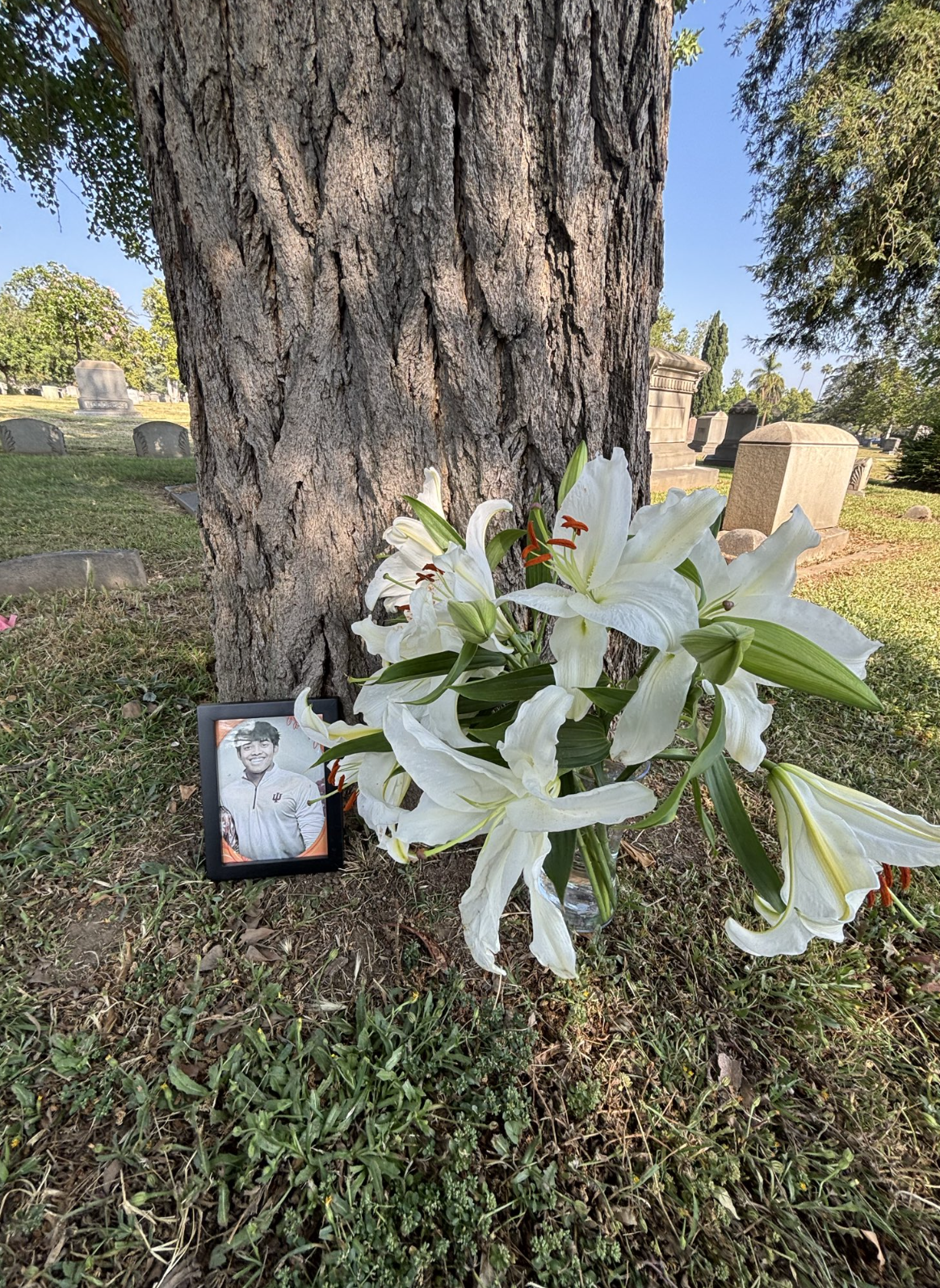
Memorial at a tree in a cemetery: a framed photograph of a young man and white lilies in a vase.

Thanks to Tuyako for discussing this poem with me.

Schur's Lemma

May 9, 2026

Irreducibility forces equivariant maps to be isomorphisms or zero.

An ordinary linear map T:VWT : V \to W can behave differently on different parts of VV; it might kill one line, preserve others, shift some lines, and collapse everything else.

A GG-equivariant map has much less freedom. It must preserve:

T(gv)=gT(v) T(g \cdot v) = g \cdot T(v)

or in other words, be GG-linear. TT sends the orbit of vv compatibly to the orbit of T(v)T(v).

When VV and WW are irreducible, they have no nonzero proper GG-invariant subspaces. However, the kernel and image of an equivariant map are automatically GG-invariant subspaces.

Example 1.1 (Why kerT\ker T is GG-invariant). Let T:VWT : V \to W be equivariant, and suppose vkerTv \in \ker T. Then, T(v)=0T(v) = 0. To show that kerT\ker T is GG-invariant (i.e., show gvkerTg \cdot v \in \ker T), we take any gGg \in G; since TT is equivariant,

T(gv)=gT(v)=g0=0 T(g \cdot v) = g \cdot T(v) = g \cdot 0 = 0

implying gvkerTg \cdot v \in \ker T, and kerT\ker T is a GG-invariant subspace of VV. (Equivariance implies that if TT kills vv, then TT kills the entire orbit of vv.)

Example 1.2 (Why imT\operatorname{im} T is GG-invariant). Let wimTw \in \operatorname{im} T. Then, there exists a vVv \in V such that T(v)=wT(v) = w. Then,

gT(v)=gw    T(gv)=gw g \cdot T(v) = g \cdot w \implies T(g \cdot v) = g \cdot w

implying gwimTg \cdot w \in \operatorname{im} T, and imT\operatorname{im} T is a GG-invariant subspace of WW.

Hence, to find VV or WW submodules we can find an equivariant map TT; kerT\ker T and imT\operatorname{im} T are GG-invariant subspaces.

What irreducibility does to kerT\ker T and imT\operatorname{im} T.

Suppose VV is irreducible and T:VWT : V \to W is an equivariant map. We know kerTV\ker T \leq V; since VV has no proper nontrivial GG-invariant subspaces, kerT={0}\ker T = \{0\} or kerT=V\ker T = V. Note that if kerT=V\ker T = V, then T=0T = 0; this usually won’t happen as we constrain TT to be a nontrivial equivariant map.

Suppose WW is irreducible and T:VWT : V \to W is an equivariant map. We know imTW\operatorname{im} T \leq W; since WW has no nontrivial proper GG-invariant subspaces, imT={0},W\operatorname{im} T = \{0\}, W. If imT={0}\operatorname{im} T = \{0\}, then T=0T = 0. Hence, if WW is irreducible, then either T=0T = 0 or imT=W\operatorname{im} T = W.

Now, suppose again V,WV, W are irreducible, and 0T:VW0 \neq T : V \to W is equivariant. From irreducibility of VV, we conclude that kerT={0}\ker T = \{0\}; it follows that T(v1v2)=0    v1v2=0T(v_1 - v_2) = 0 \implies v_1 - v_2 = 0 for any (v1v2)V(v_1 - v_2) \in V. By linearity, this implies T(v1)T(v2)=0    v1v2=0T(v_1) - T(v_2) = 0 \implies v_1 - v_2 = 0. Hence, T(v1)=T(v2)    v1=v2T(v_1) = T(v_2) \implies v_1 = v_2, implying TT is injective.

Similarly, from irreducibility of WW, we conclude imT=W\operatorname{im} T = W, implying TT is surjective. Hence, TT is an isomorphism, and VWV \cong W.

Example 1.3 (Trivial representation to sign representation). Let G=C2={e,s}G = C_2 = \{e, s\}. Let V=CV = \mathbb{C} be the trivial representation sv=vs \cdot v = v and W=CW = \mathbb{C} be the sign representation sw=ws \cdot w = -w.

We know every linear map T:VWT : V \to W has the form T(v)=avT(v) = av for some aCa \in \mathbb{C}. For equivariance, we require

sT(v)=T(sv)    T(v)=T(v)    av=av    a=0 \begin{aligned} s \cdot T(v) = T(s \cdot v) &\implies -T(v) = T(v) \\ &\implies -av = av \\ &\implies a = 0 \end{aligned}

Hence, T=0T = 0 is the only equivariant map from VV to WW (homomorphism, i.e. map respecting the GG action on VV and WW); this means HomCC2(V,W)={0}\operatorname{Hom}_{\mathbb{C}C_2}(V, W) = \{0\}.

We could have gotten this without computation through Schur’s Lemma. Since VV and WW are irreducible (as dimV=dimW=1\dim V = \dim W = 1), any equivariant map between them must be an isomorphism or 0; the trivial and sign representations are not isomorphic, so T=0T = 0, and HomCC2(V,W)={0}\operatorname{Hom}_{\mathbb{C}C_2}(V, W) = \{0\}.

(If the representations were unfamiliar, then we would have to do the T(gv)=gT(v)T(g \cdot v) = g \cdot T(v) check.)

Example 1.4 (Trivial representation to itself). Now, let VV and WW be the trivial representation. Then, T(v)=avT(v) = av for aCa \in \mathbb{C}, and

T(sv)=sT(v)    av=av T(s \cdot v) = s \cdot T(v) \implies av = av

so all nonzero maps of TT are isomorphisms; in fact, they are scalar maps, and HomCC2(V,W)={Ta(v)=av:aC}\operatorname{Hom}_{\mathbb{C}C_2}(V, W) = \{T_a(v) = av : a \in \mathbb{C}\}.

Alternatively, by Schur’s Lemma, since VV and WW are irreducible, all equivariant maps between them must be isomorphisms or 0; the trivial representation is isomorphic with itself, so HomCC2(V,W)={Ta(v)=av:aC}\operatorname{Hom}_{\mathbb{C}C_2}(V, W) = \{T_a(v) = av : a \in \mathbb{C}\}.

Equivariant endomorphisms of irreducible representations are scalars.

Let VV be a finite-dimensional irreducible complex representation, and let TEndG(V)T \in \operatorname{End}_G(V) (so TT is equivariant). Because VV is finite-dimensional over C\mathbb{C}, TT has an eigenvalue λC\lambda \in \mathbb{C} (n×nn \times n C\mathbb{C}-valued matrices have nn eigenvalues). Define S=TλIS = T - \lambda I.

First, we show SS is equivariant. In other words, we show S(gv)=gS(v)S(g \cdot v) = g \cdot S(v), or (TλI)(gv)=g(TλI)(v)(T - \lambda I)(g \cdot v) = g \cdot (T - \lambda I)(v). By linearity, (TλI)(gv)=T(gv)λI(gv)(T - \lambda I)(g \cdot v) = T(g \cdot v) - \lambda I(g \cdot v); since TT is equivariant, this equals gT(v)gλIv=g(T(v)λIv)=gS(v)g \cdot T(v) - g \cdot \lambda I v = g \cdot (T(v) - \lambda I v) = g \cdot S(v). Hence, S:VVS : V \to V is equivariant.

Since λ\lambda is an eigenvalue of TT, there exists some 0vV0 \neq v \in V such that T(v)=λvT(v) = \lambda v, implying T(v)λv=(TλI)(v)=0T(v) - \lambda v = (T - \lambda I)(v) = 0, meaning vker(TλI)v \in \ker(T - \lambda I), and ker(TλI)0\ker(T - \lambda I) \neq 0. In addition to this, since TλIT - \lambda I is equivariant and VV is irreducible, ker(TλI)=V\ker(T - \lambda I) = V, meaning TλI=0T - \lambda I = 0, so T=λIT = \lambda I.

Hence,

EndCG(V)={λI:λC} \operatorname{End}_{\mathbb{C}G}(V) = \{\lambda I : \lambda \in \mathbb{C}\}

or in other words, every equivariant endomorphism T:VVT : V \to V is a scalar.

Two examples of non-scalar equivariant endomorphisms (and thus reducible VV):

Example 1.5 (Why two eigenvalues reveal reducibility). Let

T=(2005) T = \begin{pmatrix} 2 & 0 \\ 0 & 5 \end{pmatrix}

be an equivariant endomorphism T:VVT : V \to V of some representation V=C2V = \mathbb{C}^2. We compute the eigenspaces:

E2=ker(T2I)=span{(1,0)T}E5=ker(T5I)=span{(0,1)T} \begin{aligned} E_2 &= \ker(T - 2I) = \operatorname{span}\{(1, 0)^T\} \\ E_5 &= \ker(T - 5I) = \operatorname{span}\{(0, 1)^T\} \end{aligned}

since an eigenspace of TT is the kernel of TλI:VVT - \lambda I : V \to V which is equivariant, each TT-eigenspace is GG invariant. They are neither zero nor VV so VV is reducible.

In general, a nonzero proper eigenspace of T:VVT : V \to V implies VV is reducible as it implies ker(TλI)0\ker(T - \lambda I) \neq 0. Two distinct eigenvalues are a special case forcing nonzero proper eigenspaces (since if ker(TλI)=V\ker(T - \lambda I) = V, then T=λIT = \lambda I and there wouldn’t be other eigenvalues).

Example 1.6 (A non-scalar upper triangular map). Suppose

T=(3103) T = \begin{pmatrix} 3 & 1 \\ 0 & 3 \end{pmatrix}

is an equivariant endomorphism of a representation V=C2V = \mathbb{C}^2. The only eigenvalue is λ=3\lambda = 3, and

E3=ker(T3I)=span{(1,0)T} E_3 = \ker(T - 3I) = \operatorname{span}\{(1, 0)^T\}

which is GG-invariant. Then, ker(T3I){0}\ker(T - 3I) \neq \{0\} is a nontrivial proper GG-invariant subspace of VV, so VV is reducible.

Example 1.7 (A reducible representation). Now, let G=C3=rG = C_3 = \langle r \rangle act on C2\mathbb{C}^2 by

ρ(r)=(ω00ω2) \rho(r) = \begin{pmatrix} \omega & 0 \\ 0 & \omega^2 \end{pmatrix}

Let

T=(abcd) T = \begin{pmatrix} a & b \\ c & d \end{pmatrix}

We compute all nonzero equivariant maps T:C2C2T : \mathbb{C}^2 \to \mathbb{C}^2 such that T(gv)=gT(v)T(g \cdot v) = g \cdot T(v), or in this case, if T(ρ(g)v)=ρ(g)T(v)T(\rho(g)v) = \rho(g)T(v) for all gGg \in G. Since rr generates C3C_3, we can simply check ρ(r)\rho(r):

T(ρ(r)v)=(abcd)(ω00ω2)(xy)=(aωbω2cωdω2)(xy)ρ(r)T(v)=(ω00ω2)(abcd)(xy)=(aωbωcω2dω2)(xy) \begin{aligned} T(\rho(r)v) &= \begin{pmatrix} a & b \\ c & d \end{pmatrix} \begin{pmatrix} \omega & 0 \\ 0 & \omega^2 \end{pmatrix} \begin{pmatrix} x \\ y \end{pmatrix} = \begin{pmatrix} a\omega & b\omega^2 \\ c\omega & d\omega^2 \end{pmatrix} \begin{pmatrix} x \\ y \end{pmatrix} \\ \rho(r)T(v) &= \begin{pmatrix} \omega & 0 \\ 0 & \omega^2 \end{pmatrix} \begin{pmatrix} a & b \\ c & d \end{pmatrix} \begin{pmatrix} x \\ y \end{pmatrix} = \begin{pmatrix} a\omega & b\omega \\ c\omega^2 & d\omega^2 \end{pmatrix} \begin{pmatrix} x \\ y \end{pmatrix} \end{aligned}

so we need

(aωbω2cωdω2)=(aωbωcω2dω2)    T=(a00d) \begin{pmatrix} a\omega & b\omega^2 \\ c\omega & d\omega^2 \end{pmatrix} = \begin{pmatrix} a\omega & b\omega \\ c\omega^2 & d\omega^2 \end{pmatrix} \implies T = \begin{pmatrix} a & 0 \\ 0 & d \end{pmatrix}

Schur’s Lemma does not force a=da = d, since V=(C2,ρ)V = (\mathbb{C}^2, \rho) is reducible (in fact, it is decomposable, as ρ(g)\rho(g) is diagonal for all gC3g \in C_3). We know C2=U1U2\mathbb{C}^2 = U_1 \oplus U_2, where

U1=span{(1,0)T}U2=span{(0,1)T} U_1 = \operatorname{span}\{(1, 0)^T\} \quad U_2 = \operatorname{span}\{(0, 1)^T\}

and we note that these are both GG-invariant subspaces by computing ρ(r)(Ui)Ui\rho(r)(U_i) \subseteq U_i.

Example 1.8 (An equivariant projection). Continuing with the previous representation ρ\rho, define P(x,y)=(x,0)P(x, y) = (x, 0). Then,

Pρ(r)=(ω000)=ρ(r)P P\rho(r) = \begin{pmatrix} \omega & 0 \\ 0 & 0 \end{pmatrix} = \rho(r)P

Then, kerP=span{(0,1)T}<C2\ker P = \operatorname{span}\{(0, 1)^T\} < \mathbb{C}^2, and imP=span{(1,0)T}<C2\operatorname{im} P = \operatorname{span}\{(1, 0)^T\} < \mathbb{C}^2. Hence, VV is reducible.

Birthday Party

May 2, 2026

On March 9,
He comes home,
With a birthday cake,
To wish her,
And hug her.
Only to find her,
With a rope around her neck,
Hanging from the ceiling fan.

He cuts her down,
And lays her limp body on the bed,
Propping a pillow behind her neck.
Then,
He feeds her cake,
Like she used to do
To him.

And,
Wiping crumbs off her stiff lips,
While squeezing her lifeless hand,
Tightly,
He laughs with her corpse,
'Till the sun sets.

Giving the dead girl,
Her very first
Birthday party.

100 Letters To A Dead Girl.

Thanks to Jan for feedback.

The Girl at the Phone Booth

April 22, 2026

The girl at the phone booth
Makes a call.
“Mom…Dad!” she cries.
No response at all.

As a rumbling train passes by,
She remembers Father’s final lie.
“America has a lot in store.”
Then he shoved her out the door.

When the sun begins to set,
The brave girl shivers from the cold.
She doesn’t own a jacket,
Just a worn-out shirt, filled with holes.

She puts down the phone in dismay,
And on the rock-hard ground, her head lay.
She tries dozing off, into a slumber,
Ignoring her empty stomach’s hunger.

Thanks to Nicole for reading drafts.

Introductory Notes on Tensors

April 15, 2026

What is vwv \otimes w? Let VV and WW be vector spaces. Think of vwv \otimes w as a new kind of vector built from a vVv \in V and a wWw \in W. Note that it is not an ordered pair: (v,w)vw(v, w) \neq v \otimes w. Rather, :V×WVW\otimes : V \times W \to V \otimes W is a map that is bilinear (linear for both inputs):

(v1+v2)w=v1w+v2wv(w1+w2)=vw1+vw2(av)w=a(vw)=vaw \begin{aligned} (v_1 + v_2) \otimes w &= v_1 \otimes w + v_2 \otimes w \\ v \otimes (w_1 + w_2) &= v \otimes w_1 + v \otimes w_2 \\ (av) \otimes w &= a(v \otimes w) = v \otimes aw \end{aligned}

Example (A basis for C2C2\mathbb{C}^2 \otimes \mathbb{C}^2). Let V=W=C2V = W = \mathbb{C}^2 with bases e1,e2e_1, e_2 and f1,f2f_1, f_2 respectively. Then, VWV \otimes W has basis {e1f1,e1f2,e2f1,e2f2}\{e_1 \otimes f_1, e_1 \otimes f_2, e_2 \otimes f_1, e_2 \otimes f_2\} (because these are the possible combinations of V×WV \times W for a bilinear map; note that dimVW=(dimV)(dimW)\dim V \otimes W = (\dim V)(\dim W)). Then, the basis vectors can be imagined as

e1f1=(1,0,0,0)e1f2=(0,1,0,0)e2f1=(0,0,1,0)e2f2=(0,0,0,1) \begin{aligned} e_1 \otimes f_1 &= (1, 0, 0, 0) \\ e_1 \otimes f_2 &= (0, 1, 0, 0) \\ e_2 \otimes f_1 &= (0, 0, 1, 0) \\ e_2 \otimes f_2 &= (0, 0, 0, 1) \end{aligned}

As an example, take v=2e1+3e2v = 2e_1 + 3e_2 and w=4f1f2w = 4f_1 - f_2. Then,

vw=8(e1f1)2(e1f2)+12(e2f1)3(e2f2) v \otimes w = 8(e_1 \otimes f_1) - 2(e_1 \otimes f_2) + 12(e_2 \otimes f_1) - 3(e_2 \otimes f_2)

so, in coordinate form, vw=(8,2,12,3)v \otimes w = (8, -2, 12, -3).

The tensor product of matrices. Take

A=(a11a12a21a22),B=(b11b12b21b22) A = \begin{pmatrix} a_{11} & a_{12} \\ a_{21} & a_{22} \end{pmatrix}, \quad B = \begin{pmatrix} b_{11} & b_{12} \\ b_{21} & b_{22} \end{pmatrix}

Define ABA \otimes B as

AB=(a11Ba12Ba21Ba22B) A \otimes B = \begin{pmatrix} a_{11}B & a_{12}B \\ a_{21}B & a_{22}B \end{pmatrix}

Then,

tr(AB)=tr(a11B)+tr(a22B)=(a11+a22)trB=(trA)(trB) \begin{aligned} \operatorname{tr}(A \otimes B) &= \operatorname{tr}(a_{11}B) + \operatorname{tr}(a_{22}B) \\ &= (a_{11} + a_{22})\operatorname{tr}B \\ &= (\operatorname{tr}A)(\operatorname{tr}B) \end{aligned}

so the trace of a tensor product is the product of the traces. The same diagonal-entry computation generalizes this to dimensions n>2n > 2.